How to create an Excel pivot table to analyse data?
Tutorial to create an Excel pivot table
When analysing a lot of data, it can be difficult to analyse all the information in your spreadsheet. Especially large tables with several thousand rows. Pivot tables make spreadsheets more manageable by summarising the data and allowing it to be arranged in different ways. This tutorial explains step by step how to build an Excel pivot table with text, images and a Youtube video.
Use Excel pivot tables to answer business related questions
How do you answer the question “How much does each vendor sell per year?” by looking at the sales data in the following example. Answering this question would be time consuming and complicated. This is because all the salespeople are listed in several rows and you have to add up all their sales individually. And use the subtotal command to find the total sales of each person. That’s a lot of data to go through. Here is a selection of the best shortcuts for managing pivot tables.
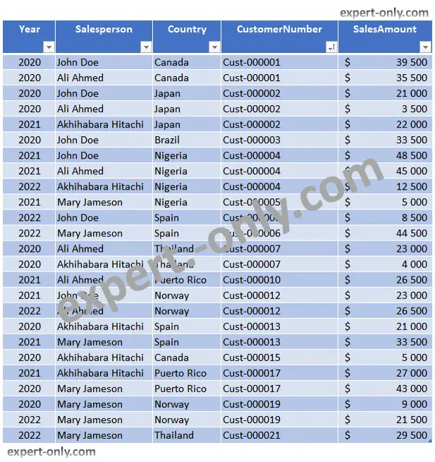
This article is an overview of the Excel Pivot Tables because it’s a sample of what you can achieve. But at the same time the essence of data crossing. The source data for the pivot table is a simple Excel table, which looks like this:
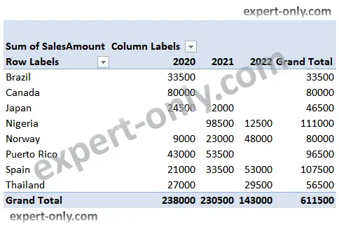
Fortunately, Excel pivot tables can calculate and summarise data in an instant in a way that is both easy to read and organise. After preparing and formatting the data, the pivot table look like this:
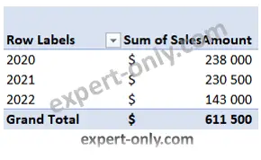
After creating a pivot table, it is possible to use it to answer different questions by rearranging the data. To answer the question “What are the total annual sales?”, modify the pivot table to look like this:
The tutorial on how to create an Excel pivot table is available in video format here:
Prepare the source data for analysis
- Select the table or cells (including column headings) containing the source data to be used.
- Go to the Insert tab and click on Pivot Table.
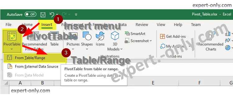
- The Pivot Table creation dialogue box will appear. Choose the appropriate parameters and click OK. In our example, Table1 contains the basic data. Configure the pivot table to be placed on an Existing worksheet.
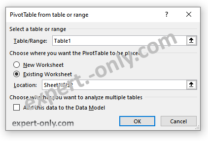
- A pivot table and a list of blank fields to select will appear in a new worksheet.
- From the PivotTable menu, select the fields to be added. Each field is simply the name one of the column headings of the original data. Check the box for each field to be added in the Pivot Table field list.
Select the fields to cross and analyse in the pivot table
In this example, you want to know the total amount of orders for each salesperson by country and by year, so check the following fields:
- Salesperson
- Country
- Year
- SalesAmount
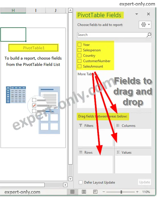
- The selected fields are added to one of the four areas below the field list. In our example, the Sellers field has been added to the Rows area and the Sales Amount field has been added to the Values area. If the area is not satisfactory, move a field to a new area by clicking on it.
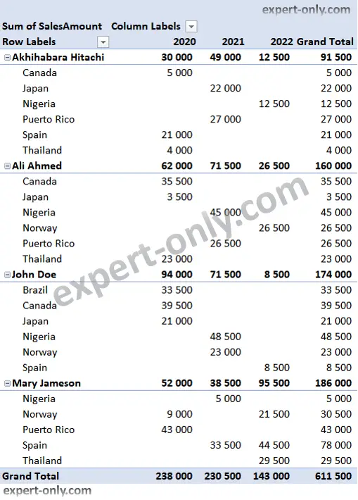
- The pivot table is used to calculate and summarise the selected fields. In our case, the pivot table shows the sum of orders for each salesperson, broken down by country and by calendar year.
- Sort the data in a pivot table like any other spreadsheet. To do this, use the Sort and Filter command in the Home tab. It is also possible to format the figures in a custom way.
- For example, change the formatting of the numbers to indicate a currency (Monetary), such as US Dollars ($) or Euros ($). Keep in mind, however, that some arrangements may disappear after changing the structure of a pivot table.
To modify the data in the source file, the pivot table will not be edited automatically. To edit it manually, select the pivot table and go to Analysis -> Refresh.
In our example, the pivot table answers the following question: What are the total sales for each vendor by country and year? Now, to ask a new question: What is the total annual sales for each country? Simply change the field in the Rows area to leave only the years.
The Excel pivot table makes it easy to cross-reference data
One of the best things about pivot tables is that you can quickly rearrange the data. This allows you to take a fresh look at the spreadsheet. Manipulating data can help answer different questions. And also allow you to experiment with new data or future projections to allow you to deduce new trends and patterns. To go further in the data analysis journey, here is a selection of the best Excel shortcuts to manage pivot tables.

