Create an Excel table from a data area.
Step by step guide to create an Excel table to manage data and sort, format and filter its columns.
In today’s data-driven world, organizing and presenting information effectively by learning how to create an Excel table is essential. Microsoft Excel, a powerful tool in the world of data analytics, offers the feature of Tables to make data presentation and manipulation much more intuitive. Creating an Excel table is not only about giving your data a neat appearance; it also provides dynamic ranges, easy filtering, and sorting.
Ready to transform your plain data into a structured Excel table? Then easily filter it? First create the required rows and columns. Fill the table with data and turn it into a table with headers. In the form of a table, it is possible to sort and filter the data easily. An Excel table is very similar to a data table, the type of object most commonly used by database professionals.
1. Create a new Excel file
The first step of course if to cerate a new XLSX file. Then add the columns. In this example, it is monthly financial data. It could be actuals till the current date (March 2022) mixed with the budget forecasting for the next months.
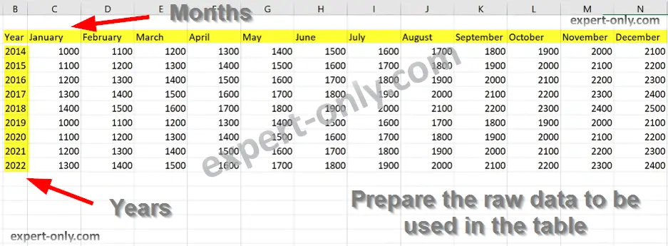
2. Generate the list of months and years
To generate the rest of the list of months in words, select the two cells January and February. Click on the small cross and hold then drag the mouse to December. The result is one year column and twelve month columns.
Then add the years from 2014 to 2022 in the Year column.
This short tutorial is available in a four minutes video format here:
3. Duplicate the excel data rows to fill the table
3 – To duplicate the rows, select the first row from January to the Total column. Then drag down as shown in this screenshot. This area of raw cells, the source of the table, is not filtered or formatted.
The following steps shows how to format the Excel table to sort the data.
4. Select the data area to transform to an Excel Table
To technically create the table follow this steps:
- Select all contiguous cells by clicking on the top left cell and use the shortcut CTRL + A to select all the data. This Excel table or area is the table, without formatting.
- Under Home, choose the option Format as a table. Choose the colour and style of the table, here it is a Blue table.
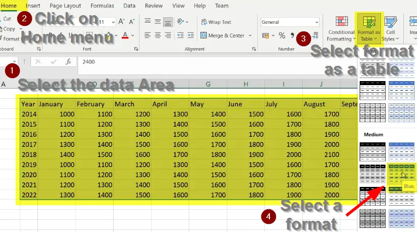
- Then, check the option My table has headers, to indicate to take into account the pre-existing headers. This action will not add any row to the table.
5. Add the totals row
Now add the totals row to obtain the grand total with all the years:
- Right-click on the Excel table
- Then choose Table
- And finally select Totals line.
The result is a formatted Excel table. It is possible to sort the cells, for example by year or to select only the year 2021 for example.
6. Use an Excel formula to calculate the sums
8 – Adding the annual total with a formula. To have the Yearly line Total column on the right, use a simple Excel formula. The Excel formula in the cell uses the SUM function:
=SUM(Table1[@[January]:[December]])
To facilitate the creation of the formula, write the SUM function in one line and then select the first row of amounts from January to December. Then make the selection slide to the last line of the data. Note: for a more sober display, deactivate the grid on the Excel tab. To do this, in the top menu of Excel, under View, uncheck the Grid option.
Finally, this short article explains how to create an Excel table to sort and filter data. To go further , here is how to manage common errors from Excel formulas like VALUE, NA or DIV0.