Excel tables are very useful to analyse and compute financial data with formulas. Sometimes a table is provided in a format that is not practical in lines; so you need them in columns. This tutorial explains step by step how to pivot the Excel table rows into columns.
How to pivot Excel table rows into columns?
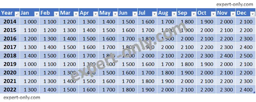
It’s really simple. You just need to select the area you want to rotate, in our example it is an Excel table with financial amounts and months. On the other hand, the special paste of the copied data is the Excel option to rotate the rows into columns.
To go faster, the MS Office tutorial is also available in video format:
Here are 3 simple steps to rotate rows into columns in Excel
- Select the rows to pivot
- Copy the rows with CTRL + C for example
- Paste the rows to be rotated, with the special paste option: Transpose.
In fact, here are the details of the three steps with screenshots to transpose the rows of the Excel table into columns.
1 – First of all, select the whole area to be rotated in the Excel sheet. With the mouse or the arrows if it is a large area. Or with the shortcut CTRL+A for a table.
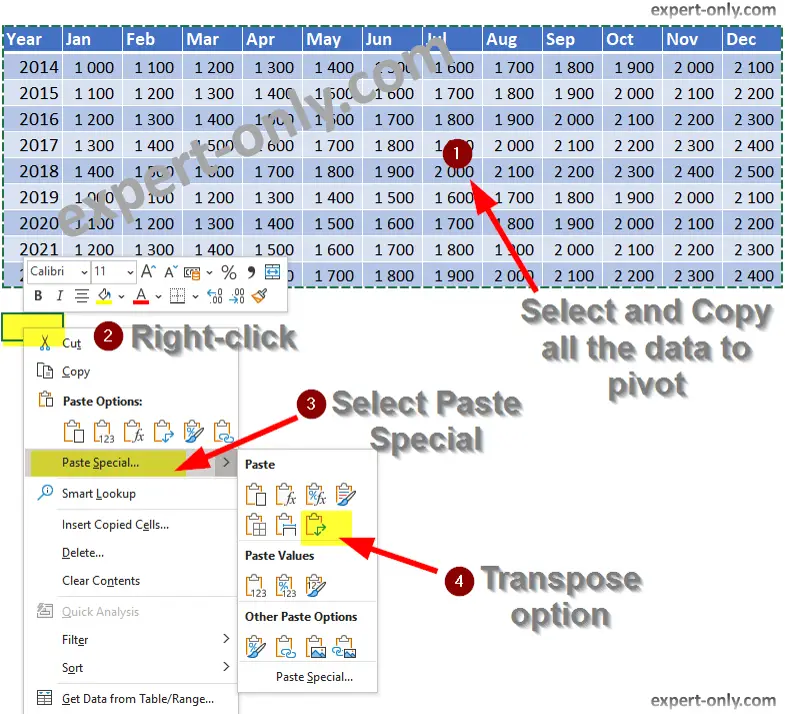
2 – Then copy the table to be rotated with CTRL+C or right-click and Copy.
- Then right-click, select Paste Special, then Transpose, as shown in the image below.
Result: The contents of the table or rows are transposed to the new location. The months are now in columns, and the different amount types are on the column headers of the new table.
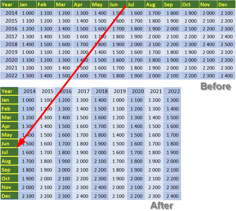
As a result, Pivoting Excel rows into columns is quick using Excel’s native transposition.
Note that this article is about how to pivot an Excel table and it is not about the Excel Pivot table.
Tables are one of the most important features of Excel. They allow you to organize data in a spreadsheet and make it easy to compare different sets of information. In this article, we will show you how to create a table in Excel by designating columns and rows.
Pivot tables are a data analysis tool that allows you to summarize and analyse your data in different ways. They can be created from by using the Pivot Table button on the Data tab of the Excel ribbon.
Another tutorial about the latter is available to learn how to build a pivot table from an Excel data table.
Excel is a part of Office 365 suite
Excel is available at very affordable rates and allows you to take advantage of other services. In particular when it is included in an Office 365 package, recently renamed Microsoft 365. These annual offers allow you to benefit from updates and new features.
Indeed, at the beginning of 2021, at the time this article was updated, the Microsoft 365 Personal offer is available at $69.99 per year, including tax. And this is the offer I subscribed to. Or $6.99 per month, that is $83.88 incl. tax per year. This offer includes 60 minutes of Skype communication per month. OneDrive storage of 1TB or 1000GB completes the offer.
To conclude, Excel tips make office work much more efficient. For example, this tip allows you to select an entire Excel column with a simple shortcut. It allows you to manipulate very large files, i.e. several thousand rows.


Be the first to comment